Introducing MIDAS
MIDAS, the Micro-Imaging Dust Analysis System, is a unique instrument that flew onboard the Rosetta orbiter. It works by exposing small (1.4 x 2.4mm) slightly sticky targets to the dust environment around the spacecraft. After (hopefully!) collecting dust, the target - which is mounted on the circumference of a wheel which can be both rotated, and translated along its axis - is moved in front of one of sixteen cantilevers. Each of these cantilevers has a 10 µm long sharp tip mounted at its end. This is the sensing element of the Atomic Force Microscope (AFM). The cantilever array is, in turn, mounted on an XYZ stage which can move the tip over the target (and sample) with high precision. The schematic diagram below shows the key components of the instrument (minus the electronics):

There are two main modes of operation:
- Contact mode - the cantilever is physically in contact with the sample, which is detected by a bending of the cantilever and,
- Dynamic mode - the cantilever oscillates close to its resonance frequency, and the sample is detected by a shift of the resonance frequency of the coupled tip-sample system (which interact with each other by van der Waals and, possibly, other forces). Since MIDAS is an amplitude-modulated AFM, the driving frequency is kept constant, and the shift in resonance is recorded as a change in the measured amplitude.
In both cases there is a slight different from the operation of a terrestrial AFM. Rather than rastering continually over the surface, tracking it with a fast feedback loop, MIDAS approaches each pixel position separately and, on reaching the surface, retreats by a “retraction height” before approaching the next position. This is overall a safer mode, especially when using amplitude AFM in a vacuum (the Q factor of the cantilevers is high, and a feedback system would be tricky) but makes operations rather slow; images can take hours, or even days, to produce.
In this post we’ll discuss basic retrieval of data and display of the scans in 2D and 3D. To fully understand the data a deeper look is needed, but we’ll save that for later posts!
For further details about the instrument, take a look at the MIDAS chapter in the 2007 special issue of Space Science Reviews (DOI: 10.1007/s11214-006-9040-y), a copy of which can be found in the data archive here. If that still isn’t enough, you can find lots of gory technical detail in the MIDAS User Manual. Finally, for details of how the data are stored in the archives, see this document.
The MIDAS dataset
Several datasets are already available in the Rosetta section of the Planetary Science Archive (PSA) and the remaining data are either under review or being processed.
The Archive InterOperability Subsystem
I used the opportunity of writing this post to try and access data via the PSA’s Archive Interoperability subsystem, which provides (limited) programmatic access to the entire archive using the Planetary Data Access Protocol.
Data can be retrieved via the PAIO by encoding the query in the URL. For example, to retrieve all of the MIDAS (INSTRUMENT_ID=MIDAS) datasets (RESOURCE_CLASS=DATA_SET) at comet 67P (TARGET_NAME=67P/CHURYUMOV-GERASIMENKO 1 (1) as an HTML table (RETURN_TYPE=HTML) you can simply build a URL like this. The result of this query is the table below, showing two datasets, ESC1 and ESC2 (the first two periods of the escort phase - after Rosetta arrived at 67P), at the time of writing this post:

If instead one sets RETURN_TYPE=VOTABLE then a VOTable object is returned which, for example, the astropy.io.votable module can read. In the Jupyter Notebook accompanying this post I use this and the requests and pandas modules to query the data sets and products and sort and filter them. Once a particular data product has been located, a separate request can be made to grab the data themselves (returned as a zip containing the product and associated label).
Note: it seems that the PAIO truncates keywords at 30 characters, such that the target name for 67P, which should be 67P/CHURYUMOV-GERASIMENKO 1 (1969 R1), has to be set as 67P/CHURYUMOV-GERASIMENKO 1 (1.
The data
For this post I’ve chosen to concentrate on three images used in a recent paper, Aggregate dust particles at comet 67P/Churyumov–Gerasimenko. The meta-data for these images, including the PSA filenames, are included in Extended Data Table 1:

The actual images from the paper can be viewed online as Figure 1, Figure 2 and Figure 3, so that you have something to compare to!
From this table, we can see that the images were acquired between January and the end of April 2015 and as the dataset query above shows, these images are split between the ESC1 and ESC2 deliveries. Be aware that this does not mean that any dust was collected at this time! For that, you have to look at the exposure history of a given target and compare scans taken before and after a given exposure. But for now just trust me that the images we will look at contain cometary dust!
If you want to directly grab the data from archive, I’ve linked it below (note that these links are to the NASA PDS Small Bodies Node mirror, not directly to the PSA since some browsers (Chrome at least) cannot directly access the PSA via FTP):
- IMG_1509813_1512600_054_ZS (ESC2)
- IMG_1507001_1508813_005_ZS (ESC2)
- IMG_1501323_1504200_013_ZS (ESC1)
Data format
As all ESA missions, Rosetta data are archived in PDS format - in this case PDS3. I won’t go into detail here; a previous blog post gives a nice introduction. For now let’s just look at the image data. If you’re accessing via FTP, you want the DATA/IMG folder - if you’re using the AIO then filter products by those with names starting IMG_.
The .IMG files are actually already written in an AFM format, the BCR format described here. So in fact you can use MIDAS data without any messing around with Python or PDS - just download the free and open source AFM software Gwyddion and away you go. If you have Gwyddion and rename the files to have a .BCR extension, then your file manager will also build thumbnails for you so you can easily browse them (at least on Mac/Linux). Here is an example of what you get “out of the box” loading one of these files - display in 2D/3D, statistical analysis, line profiles and much more:

If you browse the .IMG files you will notice that the names end in a two-letter code. This specified the data channel. In a single image MIDAS can store a variety of data types, not only the topography (labeled as ZS, for Z set point) but a phase signal (PH) and many others. For now, we will only look at the fundamental topography data - so you can also filter product names ending in _ZS.
But let’s assume we want to look at the data in Python… As described above, MIDAS makes point approaches to the target/sample at regular positions in a rectangular grid and records the extension of the Z piezo when the surface is detected. The primary MIDAS data product are thus regular height fields, with images sizes in both X and Y which are always multiples of 32, in the range 32..512.
The BCR format of the MIDAS data assumes a 2048-byte ASCII header followed by a series of 16-bit integer binary values. The header values are in = separated key/value pairs, the most useful of which are:
- xpixels/ypixels: defines the number of pixels in the image,
- xlength/ylength defines the scanning range in the given unit and
- bit2nm is the scale factor for scaling the integer height data to nm.
Note: most of these data are also available in the detached header of the image file (i.e. the .LBL file), but xlength and ylength are missing - this will be fixed in later re-deliveries. So for now this has to be read from the BCR header.
Viewing the data
2D plots
In the code below, the values are simply read into a numpy array and the integer values multiplied by the scaling factor to get a value in nanometres. Using the xlength and ylength values, matplotlib can be used to show these height fields (click to open each at full res in a new tab):
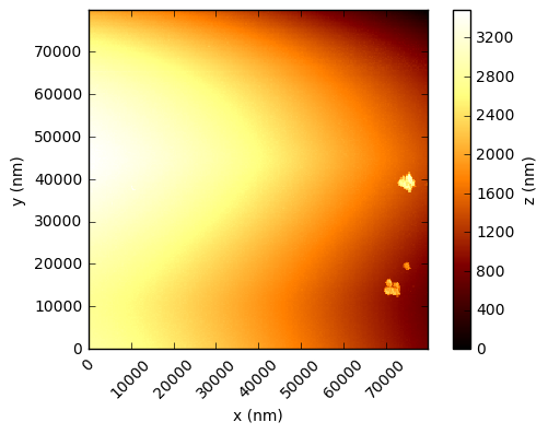
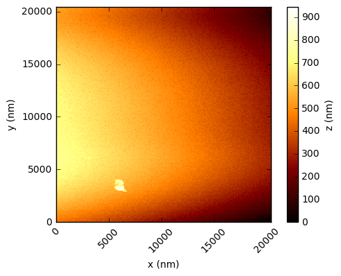
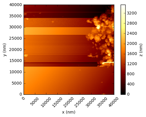
You should see that this gives a similar result to the figures in the Nature paper, which are a processed crops of these same scans. There are a few things to note - in the first two figures, the target substrate appears not to be flat - this is due to a combination of the slope between the XYZ scanner and the target, and drifts (due to temperature, for example). Knowing that the substrates are in reality rather flat, a standard AFM technique is to mask out the particles and either fit a plane, or polynomial, surface and subtract this from the data.
3D interactive plots
Two dimensional plots are great, but since the data are in 3D we should also display them in all their glory! We’ve already covered reading the data into an array, so now I’m just going to use plotly to render an interactive 3D surface plot.
Animating the data
Since MIDAS generates 3D data, it is of course fun to think about some “flythrough” animations. The video below shows such an animation made using the 3 images discussed so far. To make these the image data were simply converted to VTK format (in fact a structured grid legacy ASCII VTK file) and then ParaView used to produce animations in which the virtual camera is moved around the scene.
The code
Below you can find a Jupyter Notebook which grabs one of the images used in this tutorial and displays it using matplotlib. It’s quite “long winded” since everything is explicitly coded. Hopefully it gives you some ideas, and I’ve tried to be liberal with comments!
Next steps
There’s a lot more to fully understanding MIDAS data than simply viewing the images. Other topics that I will try to cover in future include:
- X/Y/Z calibration using the on-board calibration targets
- Understanding the frequency scans (in dynamic mode)
- Housekeeping and event history data
If you have questions, or want more details you can ask me via Twitter or follow @RosettaMIDAS!