ChemCam is a laser-induced breakdown spectroscopy instrument used to derive chemical composition by ablating targets from stand-off distances of up to 7 meters. Or as I prefer to describe it: ChemCam zaps rocks with a laser to figure out what they’re made of. Since ChemCam can be used quickly and from a distance, it is used almost every day on Mars. Curiosity has been exploring Gale crater for 1554 sols and has collected more than 400,000 ChemCam spectra! It’s a huge trove of data, of a type that has not been collected on any previous planetary mission, so it can be intimidating to work with, but I hope this post will serve to demystify it a bit! I’ll start by describing LIBS, then walk you through how we process the spectra and derive compositions. For more detail, you can refer to the presentations that we presented at our data user workshop at LPSC in 2015.

How it works

Laser-induced breakdown spectroscopy (LIBS) works by concentrating intense pulses of laser light on a target, so that a small amount of the target is “ablated” and turned into a plume of plasma. That plasma plume gives off light that can be passed to a spectrometer and analyzed to identify the emission lines of chemical elements in the target. Under normal Earth-like atmospheric pressure, the LIBS plasma plume can’t expand very much, while under hard vacuum conditions the plasma plume is unconfined and expands really fast. In both cases, it is not especially bright. On the other hand, Mars is an ideal environment for LIBS because its thin atmospheric pressure is “just right,” giving nice bright sparks. As a bonus, the shockwave formed by the expanding plasma has enough force to clear away the pervasive dust that covers everything on Mars. Since LIBS works by ionizing the target material, it theoretically can detect any element that has emission lines (in other words, all of them). However, it is most sensitive to elements that are easy to ionize and have nice, bright lines. That means ChemCam is particularly good at identifying alkali and alkali earth metals (even very light elements like Li). It is least sensitive to elements like chlorine and sulfur that are harder to ionize, though they are still detectable at high enough abundances. ChemCam uses three spectrometers to span a spectral range from 240 nm to 850 nm where most common elements have emission lines. As shown below, it is possible to say quite a lot about a target just by looking for certain diagnostic lines in the spectra. To help with this sort of analysis, you can use the NIST spectral database, or download this handy tool developed by Agnes Cousin (also see this presentation for details on how to use the tool).

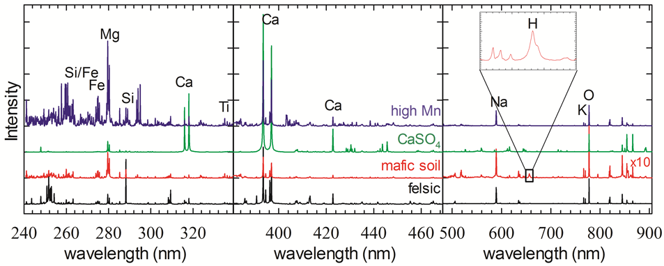Fig. 1: Example ChemCam spectra from Mars of targets with very different compositions.

A Typical Observation

Before we discuss how the data are processed, it’s worth talking about how a typical ChemCam observation is conducted. For LIBS to work, the laser light must be focused on a small enough spot to generate plasma. The ChemCam spot size varies slightly depending on distance to the target, but is less than 0.6 mm. To get a better idea of the variability of composition in a target, we usually analyze multiple locations or “points” on the target. These points are organized in a grid (e.g. 3x3) or a straight line (e.g. 1x10). At each point, we typically use 30 laser shots which allows any dust to be cleared away (usually within the first 5 shots) with a good number of spectra left over to average together to get a good measurement. The spectra can also be analyzed individually to look for variations with depth as the layer ablates away the upper few microns of the target. ChemCam spectra are grouped together by point, so for a 1x10 observation of a target, there will be 10 files, each of which contains 30 spectra (one per shot). For each point, we also collect a “passive” or “dark” spectrum, where the laser is left off and the spectrometer just collects reflected sunlight.

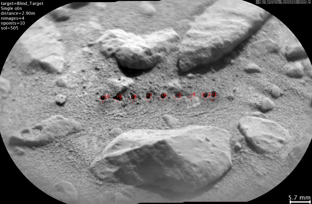Fig. 2: Example RMI mosaic showing LIBS pits in soil on Mars.

Along with the spectra, a typical observation also includes Remote Micro Imager (RMI) images. The RMI uses the same telescope that focuses and collects the laser light, and provides a high-resolution view of the target. By taking an RMI image before and after doing LIBS, it is possible to see the marks left by the laser and understand the geologic context of each chemical analysis. Depending on the number and spacing of the analysis points, additional RMI images are sometimes interspersed between LIBS analyses. Each ChemCam file name contains a lot of information about the file. The figure below spells out what each piece of the filename means:

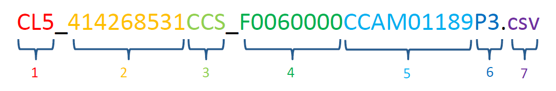
1. Type of data: CL5 = LIBS spectra, CL9 = Passive/”dark” spectra, CR0 = RMI image, CL0 = Averaged passive/”dark” spectra.
2. Spacecraft clock: this is the time in seconds from a certain reference date that the observation was collected. It serves as a unique identifier for each observation.
3. Processing level: EDR = raw data (“experimental data record”), RDR = Level1a (“reduced data record”), CCS = Level 1b (“cleaned calibrated spectra”), MOC = Level 2 (“major oxide calculation”), PRC = processed RMI.
4. Flight software version
5. Sequence ID: The first two digits after “CCAM” indicate the number of the observation for the given sol. The next three digits indicate the sol number. For sols after 1000, these three digits are the final three digits of the sol number. So sequence 2 on sol 1423 would have the ID “CCAM02423”.
6. Processing version: Always use the highest number available.
7. File extension

Level 1 Data Processing

Level 1 processing starts with the raw data (experimental data record” or “EDR”) and cleans up the spectra so that they can be used for analysis. The first step is to subtract the “dark” spectrum to isolate just the signal from the plasma. Next we use an undecimated wavelet transform to remove noise from the spectrum. (For more detail on this, refer to Wiens et al., 2013 and this presentation) After denoising, we apply a wavelength calibration. Since LIBS spectra are made up of narrow atomic emission lines, it’s important for the wavelength to be calibrated very accurately. This is done by analyzing the Ti plate calibration target on Mars when the instrument is at different temperatures and comparing with Ti measurements from the lab on Earth. This results in a wavelength shift as a function of temperature for every pixel that is applied to get the spectra lined up correctly. LIBS spectra have a continuum signal caused by Bremsstrahlung emission and ion recombination in the plasma that doesn’t contain much information about the target material, so we typically remove the continuum. This is done in a manner similar to the denoising algorithm by using a wavelet transform to split the signal up into different wavelet scales, then identifying local minima at each scale. A spline fit to the local minima gives the continuum, which is then subtracted to leave just the emission lines. Again, details on the procedure are in Wiens et al., 2013 and in this presentation from the data workshop. The amount of continuum relative to the emission lines in ChemCam spectra is somewhat related to the distance to the target, so removing the continuum partially corrects for distance effects.

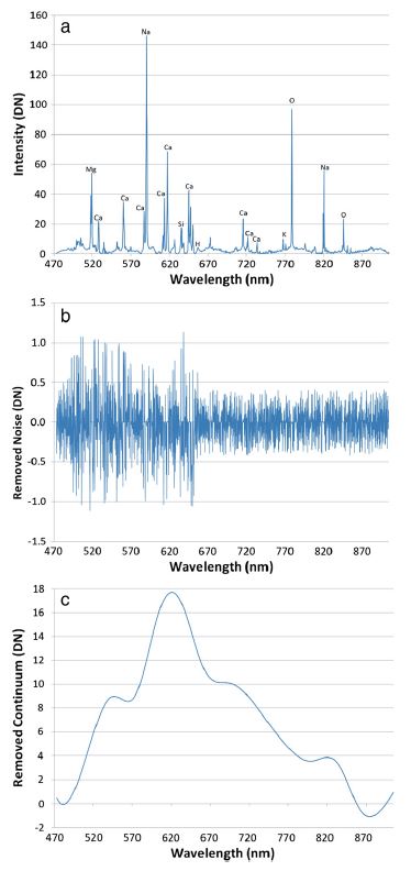
Fig. 3: Figure from Wiens et al., 2013 showing noise and continuum signal removed.

Once the continuum is removed the spectrum is at the “reduced data record” (RDR) stage. From there, we convert the data from counts to photons by applying an “instrument response” correction based on laboratory observations of standard light sources, along with some geometric factors related to the distance, spot size, spectrometer field of view, etc. At this point the spectra are in good shape and are ready to be used for further analysis. Spectra that have been processed to this point are called “cleaned, calibrated spectra” and have “CCS” in the file name. Often, before proceeding to the data analysis stage, other preprocessing steps such as masking and normalization are applied. Masking is simply the process of excluding portions of the spectrum. We do this primarily to remove the edges of the spectral ranges where the instrument response is not as good, causing more uncertainties in the data. Normalization generally involves dividing each spectrometer by its total integrated intensity or dividing the full spectrum by the total intensity across all three spectrometers. Normalization helps to limit fluctuations in the data.

Qualitative Analysis

CCS spectra can be used directly for qualitative analysis by identifying certain emission lines as mentioned above. Other commonly-used qualitative methods for visualizing ChemCam LIBS spectra are Principal Component Analysis (PCA) and Independent Component Analysis (ICA). PCA is a widely used method for reducing the dimensionality of data but I’ll briefly describe how it works. You can think of a ChemCam spectrum, which has 6144 different spectral channels, as a point in 6144 dimensional space. (Or more likely, you can’t, because humans can’t really visualize more than three dimensions! But bear with me…) A bunch of spectra create a cloud of points in this high-dimensional space, and what we want to do is visualize that cloud in a more manageable number of dimensions. PCA works by finding the axis through that high dimensional space along which the point cloud varies the most. This axis is a “principal component”, and can be summarized as a “loading” which is a vector of coefficients (one per spectral channel) that gets multiplied by the spectra to calculate a “score” that indicates where along the component axis the spectrum plots. (For the mathematically inclined, PCA loadings and scores are analogous to eigenvectors and eigenvalues.) PCA loadings resemble LIBS spectra with some emission lines that are negative instead of positive, indicating an inverse correlation. The process continues by finding another axis, perpendicular to the first axis, along which the point cloud has the next-highest amount of variation. This is the second “principal component” and likewise each spectrum gets a score. This process can be repeated as many times as there are dimensions in the original data, but in general, the vast majority of the variation in the data can be explained by using just a few principal components. The scores can be plotted against each other to visualize spectral variations in two dimensions.

Fig. 4: Example PCA score plot and associated loadings. Points are color coded by known K2O content. Plot generated using PySAT.

ICA is conceptually similar to PCA: it decomposes the data to a smaller number of variables, but it does not require the components to be perpendicular to each other. Instead it seeks components that are statistically independent. There are several algorithms for ICA but we typically use the JADE algorithm, which results in loadings that tend to isolate the emission lines from a single element in the plasma. This means that plots of ICA scores are easier to read than PCA score plots, since each axis is basically the strength of the emission lines for one element.

Fig. 5: Example ICA score plot and associated loadings. Points are color coded by known K2O content. Plot generated using PySAT.

PCA and ICA scores are often used as the inputs to clustering or classification algorithms since they efficiently summarize most of the key information in the spectra. There are a wide variety of clustering and classification algorithms that can be used.

Quantitative Analysis

Of course, we usually want to go beyond just detecting the presence of an element in a LIBS spectrum: we want to know how much of it there is! All methods of quantitative analysis rely upon a suite of spectra for which the composition is known, so that spectral features can be related to composition. The original ChemCam training database containing spectra of 66 standards has been expanded to a diverse set of 482 standards, and is available on the Planetary Data System (PDS) here. The simplest way to get quantitative results is to use “univariate” calibration, where a single variable such as the peak area of an emission line is plotted against the quantity of the element of interest, and a calibration curve is fit to that data and used to estimate the composition of unknown targets based on their spectra. This method is most effective for minor and trace elements. Major elements can also be predicted using univariate methods, but there is often a significant amount of scatter resulting from variations in emission line strength that are due to factors (collectively called “matrix effects”) other than the concentration of that element. Multivariate calibration methods are more advanced statistical methods that use the entire spectrum rather than just a single emission line to estimate the abundance of an element. By using the full spectrum, these methods can partially counteract matrix effects, resulting in more accurate results for most major elements. The downside is that these methods are less intuitive than univariate methods. The latest ChemCam calibration uses a combination of ICA Regression and sub-model Partial Least Squares (PLS) regression to estimate the composition of targets on Mars. ICA regression is similar to univariate regression, except instead of using the peak area of a single line, it uses the ICA score corresponding to a major element to come up with a calibration curve. PLS is a widely used multivariate method that is similar to PCA in that it represents the data as a combination of several components. Sub-model PLS takes advantage of the fact that a regression model that is trained on a limited range of compositions (e.g. MgO between 0 and 5 wt.%) is generally more accurate over that composition range than an “all-purpose” regression model trained on all compositions (e.g. MgO between 0 and 100 wt.%). By using a 0-100 wt.% model in combination with several “sub-models” that specialize on smaller composition ranges, we get better results than just using the 0-100 wt.% model. You can read more about the sub-model concept here (contact me for the full manuscript). Fig. 6: Example from Anderson et al., 2016 illustrating the concept of sub-model PLS regression.

There’s a lot more involved in optimizing regression methods and estimating their accuracy, but I have already gone on long enough in this post so I will just say that for the PLS models we use multi-fold cross-validation using folds stratified on the composition of interest. If you’d like to know more, please contact me!

Getting the Data

The main place to look for ChemCam data is on the Planetary Data System (PDS). Raw data is available here and processed data is here. If you’d rather skip all of the complicated stuff above and just want the derived major element oxide compositions, they are available here. You may also want to take a look at the “master list” which contains a lot of useful metadata about all of the ChemCam observations, including indications of spectra that were excluded from the PDS due to saturation, low signal, or major element composition totals greater than 110 wt.% (this indicates a problem with one or more of the major element predictions). For RMI images, they are available on the PDS, but your best bet is to get the annotated RMI mosaics from the ChemCam website.

Working with the Data

If all of the complicated stuff above makes you want to dig in and get your hands dirty with processing your own data, then you can do that too! If you are a skilled programmer, then you can probably take the raw or CCS-processed data and run with it. However, if you want a head start, I have been working with a student on a NASA PDART-funded effort to develop a collection of code for analyzing ChemCam data (and other spectral data) called PySAT (Python Spectral Analysis Tool). It is still very much in development, but if you’re willing to put up with some bugs it may still be useful for you, and we’re constantly improving it. The “back end” code is available at this repository, and the “front end” graphical interface is available here. The GUI doesn’t yet implement everything that is possible to do with the back-end, and the back-end in turn doesn’t yet do everything that I eventually hope it will be able to. However, if you’re interested in this sort of thing, please do take a look! If you try the code and run into any issues or would like to request additional features, please get in touch with me so that we can made the code as useful as possible!

---

• ← Previous Post
• Next Post →